Life Cycle Assessment
Life cycle assessment (LCA) was developed in the 1960s within the field of industrial ecology, as a “cradle-to-grave” approach for assessing the impacts of industrial systems and manufacturing processes on environmental and human health (Horne et al., 2009). An LCA begins with an inventory of the raw materials required to produce a product and ends at the point when all those materials are returned to the earth. All inputs and environmental releases to air, water and land are determined for each life cycle stage and/or major contributing process over the product’s life span. In the early 1990s, researchers began using LCA to analyze food systems, specifically food processing and packaging. More recently, LCAs have been used to assess food crop, animal production, and biofuel feedstock systems.
Key characteristics of LCAs include:
“Cradle-to-grave” analysis.
A multidimensional approach. LCAs analyze pathways by which environmental damage occurs, based on environmental impacts. This approach assesses both immediate or local impacts (e.g., human toxicity, water use/contamination) and long-term or global concerns (e.g., global warming, depletion of nonrenewable resources).
Flexible functional units. The comparison and analysis of alternative systems is based on equivalency of service delivered. For example, instead of comparing the environmental impacts of one pound of herbicide A with one pound of herbicide B, the quantity compared would depend on the application rate over a given acreage. This normalizes the assessment with respect to the final service delivered. More than one functional unit can be used in the same analysis (e.g., CO2 emissions per acre or per pound of yield).
Subjectivity. LCAs reflect subjective decision-making, particularly with respect to the design of the analysis (scope and functional unit) and the interpretation of outcomes (Horne et al., 2009). The interpretation of trade-offs across environmental impacts depends on the setting.
Strong comparative ability. LCAs provide a strong approach for comparing specific resource inputs (e.g., fertilizer, chemicals and energy) and multiple environmental consequences.
Application of Life Cycle Analyses to Agricultural Systems Research
The use of LCA in agricultural systems is relatively new; in general, there are three ways to use LCA to evaluate agricultural systems:
Comparing life cycles for a product or service. This is the most common usage of LCA in agriculture. To compare life cycles, the scope and functional units must be consistent for all production systems. For example, organic and conventional production systems have been compared for a variety of products, including one ton of milk (Thomassen et al., 2008), one ton of bottled wine (Pizzigallo et al., 2008) and a one-kilogram loaf of wheat bread (Meisterling et al., 2009). Other studies have compared management strategies. For instance, Capper et al. (2008) evaluated the environmental impacts of rBST in dairy systems, Brentrup et al. (2004) assessed the environmental impact of varying fertilizer rates on wheat production (per ton of wheat), and Haas et al. (2001) compared milk production from intensive, extensive and organic grassland farming systems (per ton of milk).
Identifying parts of the life cycle where the greatest improvements can be made. This type of analysis entails a detailed assessment of a single product to evaluate the input requirements and environmental impacts of each stage of production through use and disposal. Landis et al. (2007) used LCA to evaluate the consequences of corn–soybean feed in terms of energy, carbon emissions, nitrogen and phosphorus flows, pesticides, and air pollutants. Through LCA, they identified the steps in grain production that account for the majority of air emissions (crop farming, fertilizers and on-farm nitrogen flows), and the steps that were less significant (seed production and irrigation). See the SARE case study (p. 76) of how one research team used LCA to monitor and develop an energy- and materials-independent dairy farm.
Comparing alternative products, processes or services. This type of analysis compares different products or processes that have the same function and is used in cases where there are distinct, interchangeable options. In other words, rather than simply comparing different production systems for specific products (e.g., orange production systems), the functional unit is broadened to compare the environmental outcomes of different products serving the same function (e.g., guavas, kiwis and oranges could be compared as a source of vitamin C). This type of analysis is very challenging and is relatively rare for agricultural systems compared to the first two applications. Examples include Eshel and Martin (2006) and Eshel et al. (2010), who examined the consequences of nutritionally sound animal-based diets versus plant-based diets consisting of similar caloric and protein contents.
Overview of LCA Methodology
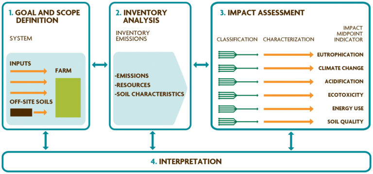
LCA consists of four distinct processes (Figure 4.4):
- Goal definition and scoping: define and describe the product, process or activity.
- Inventory analysis: identify and quantify energy, water and materials usage and environmental releases (e.g., air emissions, solid waste disposal, wastewater discharges).
- Impact assessment: assess the potential human and ecological effects of energy, water and material usage, and assess the environmental releases identified in the inventory analysis.
- Interpretation: evaluate the results of the inventory analysis and impact assessment to select the preferred product, process or service with a clear understanding of the uncertainties and assumptions used to generate the results.
(For more detailed information on how to apply LCA to agricultural systems, see EPA, 2006 and Horne et al.,2009).
LCA stage one: goal definition and scoping. Goal definition and scoping determines the purpose and expected outcome of the study, establishes the system boundaries, and defines the functional units (FU) and assumptions. System boundaries can be illustrated by a general input and output flow diagram (Figure 4.5). All operations that are part of the life cycle of the product, process or activity fall within the system boundaries. The purpose of the FU is to provide a reference unit to which the inventory data are normalized (e.g., application rates for agrochemicals are usually normalized per acre or other land-area unit). The FU varies across studies and is determined by the system boundaries, the product or processes of interest, the type of environmental impact and the aims of the investigation.
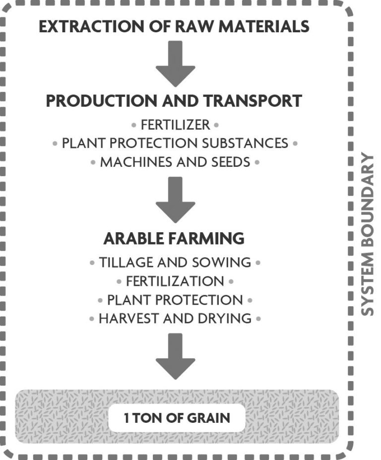
The system boundary can be defined in several ways in LCA studies comparing agricultural production systems. Brentrup et al. (2004) used LCA to determine the environmental impacts of different fertilizer management regimes in wheat production systems. They defined the functional unit as one ton of wheat; their system boundaries began with the extraction of raw materials and ended with the harvest and drying of the wheat (Figure 4.5; Brentrup et al., 2004). In contrast, Meisterling et al. (2009) compared organic and conventional wheat production using 0.67 kilograms of wheat flour as their functional unit; bread was their target product and this FU represented the amount of flour used to make a one-kilogram loaf. This latter study encompassed a larger system that included all of the steps in wheat production, harvest, transport and processing into flour. Brentrup et al. (2004), however, limited their analysis to crop production because their functional unit was unprocessed wheat grain. Other common functional units used in agricultural LCAs include the nutritional value or quality of the product and the land area required per unit of production.
Decisions about the LCA scope and functional units can determine the conclusions drawn about how management systems affect the environment. For example, in an LCA comparing three pig production systems (Basset-Mens and van der Werf, 2005), environmental impacts were expressed using two different functional units: per kilogram of live pig weight produced and per hectare of land used (including off-farm land used to produce crop-based ingredients for feed). When the systems were compared in terms of impacts per land area used, the organic and red-label systems had better performance; the relative performance of the systems was significantly different when impacts per kilogram of pig production was used as the functional unit.
LCA stage two: life cycle inventory analysis. The life cycle inventory analysis quantifies energy and raw material requirements, atmospheric and waterborne emissions, solid wastes, and other releases for the entire life cycle of a product or farming system. It is the most resource-intensive and time-consuming stage because it requires large amounts of data collection. LCA software is available for purchase and includes databases on the transport, processing and production of commonly used products such as plastic, refined metals and cardboard. Several free LCA software programs are also available (EPA, 2006); these programs contain data for processes that are not product-specific, such as general data on the production of electricity, agricultural inputs and fuel. The USDA is working to improve the accessibility, transparency and quality of the data. (See the LCA Digital Commons project led by the National Agriculture Library, www.lcacommons.gov.)
When using LCA in agricultural systems analysis, practices such as tillage frequency or application rates of pesticides or soil amendments require site-specific data. For a complete LCA, all inputs and outputs from the processes and materials used in crop production must be included. Inputs include energy (renewable and nonrenewable), water, and raw materials. Outputs include products and coproducts, emissions (e.g., the greenhouse gases CO2, CH4, SO2, N2O, NOx and CO), chemicals (e.g., nutrients, chlorinated organic compounds and other agrochemicals), biotic losses (e.g., genes or exotic organisms) to air, water and soil, solid wastes, and soil loss or degradation.
LCA stage three: impact assessment. Impact assessment evaluates the impacts of resource use and emissions identified during the inventory analysis; its purpose is to address ecological and human health effects and consequences of resource depletion. For example, an evaluation of irrigation systems might show that furrow irrigation uses more water but that disposable drip tape uses more material inputs and produces more waste. In this example, the assessment would weigh water-use efficiency against the use of fossil fuels (in the manufacture of plastic) and the generation of solid waste to determine which system had the more severe environmental impact. A complete accounting of inputs and outputs improves the capacity to compare production systems, even when the resources used and emissions generated vary across the systems or processes under study.
LCA Stage four: interpretation. Although the LCA framework is based on detailed guidelines and extensive databases, this approach relies heavily on interpretation by the research team throughout all stages (Figure 4.4). Conclusions drawn and recommendations made reflect the regional, cultural and institutional values of the individuals conducting the LCA. As a result, although the rigor and consistency of LCA analysis have improved greatly, it is still subject to interpretation. For example, in the furrow versus drip irrigation scenario described above, the importance assigned to each environmental impact is site specific and based on subjective judgment. In a region with serious water limitations, for instance, reduced demand for irrigation water could be the environmental priority, so the team might decide that the advantages of the drip system outweigh its drawbacks (e.g., increased solid waste and greater greenhouse gas emissions from the manufacture of drip materials).
Given this “situational” aspect of LCA, be very clear about the rationale and goals of an LCA, and be prepared to explain the basis for conclusions drawn. Include all data collected in the inventory stage and the impact assessment. Transparency in the methods used to collect and calculate data and in the basis for interpretation of the LCA is critical; this transparency greatly increases the potential to compare and synthesize results from different LCAs of the same product or similar production system. For example, in the case of wheat production on p. 70, the decision by two teams to use different functional units (i.e., raw wheat grain versus flour) resulted in different system boundaries, which could impact the interpretation of these two LCAs.
Strengths and Limitations of LCA
A key strength of the LCA approach is that it enables the use of a single analysis to consider multiple resources and impacts and to compare environmental consequences from local to global scales. As a result, LCA can be useful in a variety of agricultural systems research settings, from field station projects comparing multiple cropping systems, to on-farm projects conducted at the farm scale, to projects comparing agricultural systems at regional or national levels. Furthermore, LCA has a long history of application in industry and manufacturing, which has resulted in a vast amount of information relevant to agricultural systems.
The flexibility that makes LCA a compelling tool for guiding management decisions toward greater sustainability presents challenges for drawing broad, generalizable conclusions. The LCA design can affect the outcomes and conclusions, so consider all design details of each LCA before comparing results (van der Werf et al., 2007; Horne et al., 2009). Also, while detailed output from LCAs is valuable, interpreting the results can be challenging, and subjective judgments are inevitable (Horne et al., 2009). Full LCA analyses can be too complex for extension and education purposes (although some LCA output, such as energy use and carbon footprint findings, can be more accessible).
Computation of emissions is the least reliable aspect of LCAs of agricultural ecosystems, because emissions are generally from nonpoint sources and there are insufficient empirical data. Some useable data have been collected through projects such as the National Agriculture Library’s LCA Digital Commons and the National Renewable Energy Laboratory’s Life Cycle Inventory database, but significant gaps remain, especially due to the nonpoint characteristic of agricultural systems.
Lastly, LCA focuses mostly on ecological and environmental systems, although more recently LCA has been applied in a social context as well (Norris, 2015).
Ecological Footprints
Ecological footprint accounting was developed in the early 1990s (Wackernagel and Rees, 1995; Kitzes and Wackernagel, 2009) and is used to analyze human consumption of biological resources and generation of wastes in a specified ecosystem area, which is then compared to the biosphere’s productive capacity in a given year. The ecological footprint approach attempts to answer a single question: “How much of the planet’s capacity is used relative to what is available?”
Ecological overshoot: when population demand exceeds the supply or biocapacity of the environment.
The ecological footprint approach is not a predictive tool. Rather, it provides information that can be used to track changes through time and to assess past and current resource consumption. This approach has been applied to a wide assortment of scales and units of analysis (Ewing et al., 2008); perhaps the most well-known application is its use in estimating the extent of global ecological overshoot (Wackernagel et al., 1999). Ecological footprints can be calculated for individuals, groups (e.g., the population of a city, watershed or nation), and activities (e.g., agricultural production) and can be used in studies at larger scales (e.g., the watershed or foodshed).
Ecological footprints are calculated by converting the inputs required for a product or process to a corresponding area of land or water that is needed to produce the resources or assimilate the emissions associated with that product or process. The calculations usually include six land-use categories: cropland, pasture, forest, energy land, built-up land and fishing ground. These areas are converted to their global hectare equivalents using yield and equivalence factors (Monfreda et al., 2004). The equivalence factor reflects differences in productivity among land-use categories; the yield factor captures the difference between local and global average productivity of the same bioproductive land type (Monfreda et al., 2004). Each resulting global hectare is a standardized and productivity-weighted unit of global average productivity (Monfreda et al., 2004). Footprints are compared to the biocapacity of a given area; biocapacity represents the maximum available resource capacity, measured in area of bioproductive land, and varies depending on the goal of the analysis. Biocapacity is considered a threshold and is used as a benchmark for the footprint analysis (Wackernagel and Rees, 1995; Monfreda et al., 2004).
Application to Agricultural Systems Research
Ecological footprint accounting is in the early stages of application to agricultural systems. So far, it has been most commonly used to compare different production systems for a particular crop, such as tomatoes (Wada, 1993) or wine (Niccolucci et al., 2008). Wada (1993) compared the land area and energy/material inputs required to grow a thousand tons of tomatoes in hydroponic greenhouses to the corresponding requirements for high-input, field-based production. He found that per unit growing area, the greenhouses were six to nine times more productive than the field (Figure 4.6). However, when all energy and material flows were taken into account, the ecological footprint of greenhouse tomato production was 14 to 20 times larger than that of high-input field production (Figure 4.6), revealing the intensive resource requirements of heated hydroponic greenhouses.
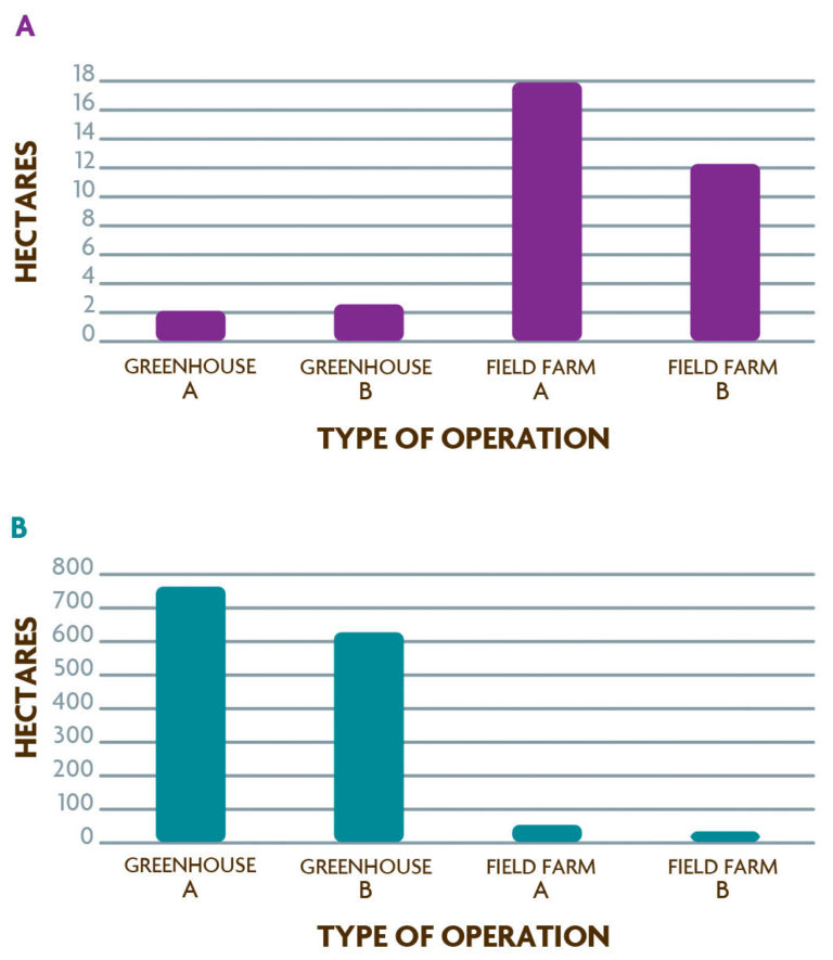
Although conventional metrics show conventional agricultural systems to be more productive on a simple yieldper- acre basis, footprint analysis reveals the opposite: these systems subsidize production through the use of nonrenewable resources such as fossil fuels. Footprint analysis often shows that greater yields per acre achieved through increased use of technology and industrial inputs actually increase the appropriated land requirements per unit of production, when all the inputs are considered. While LCA can provide similar conclusions, ecological footprint accounting integrates resource use by converting everything to land area equivalents. This can be a useful tool for communicating differences in resource use to farmers and other stakeholders who are more familiar with yield-per-acre comparisons.
Strengths and Limitations
Ecological footprint accounting has much in common with LCA. It is a data-intensive approach with a strong ecological basis for assessing the performance of an entire system. Data sets and calculation methods for ecological footprint assessments have improved greatly since the 1990s (Ewing et al., 2008) and are continuing to improve (Kitzes et al., 2009), and extensive databases and other resources are available to support these analyses.
The most notable limitations of ecological footprint accounting are in the analysis of greenhouse gas emissions and water use. Using current methodology, greenhouse gases can only be accounted for as land area required to sequester CO2, so all greenhouse gases must be converted to CO2 equivalents. Also, although water is a limited resource, it is not derived from ecosystem production and is not accounted for in the land-area conversions. Researchers are working to resolve these key problems and other limitations (Kitzes et al., 2009; Wackernagel, 2009). Footprint analyses cannot account for some aspects of environmental sustainability, such as resource depletion outside the biosphere (for example, the mining of metals) and the environmental impact of toxins and materials that do not decompose. These impacts cannot easily be converted to use of a portion of the biosphere. In systems where resource depletion and toxic outputs are important, LCA can complement footprint accounting.
Despite its limitations, ecological footprint accounting is a valuable tool for evaluating systems at a variety of scales—farm, regional, national and global—and it allows per-capita comparisons. Furthermore, footprints eliminate the subjective judgment required at many stages of LCA by converting resource use and consequences to a single quantitative unit. Footprint analyses share a common basis and set of calculations; as a result, all ecological footprint assessments can cite the same methodology, and broad comparisons can be made without checking the underlying assumptions and calculations. This ability to compare widely divergent systems using the same framework on the same terms is a strength of footprint analysis that complements the application-specific nature of LCA.
Carbon Footprints
Previously, efforts to study greenhouse gas reductions in agricultural systems centered only on the sequestration of carbon as soil organic matter (Lal et al., 2007). Since agricultural production generates significant greenhouse gas emissions, however, a full accounting of both carbon emissions and sequestration is needed. The net balance between emissions and absorption is the “carbon footprint” and includes production of all greenhouse gases, including N2O and CH4, which are converted to CO2 equivalents. Carbon footprints have been used to compare different types of crops and agricultural production systems, such as organic versus conventional (Hillier et al., 2009) and historical versus contemporary dairy production (Capper et al., 2008). They have also been used to compare the greenhouse gas consequences of different human diets (Stehfest et al., 2009).