
Systems experiments, by the nature of their design and goals, have multiple confounding factors that cannot be easily separated (Teasdale and Cavigelli, 2010). This means that a mixture of statistical approaches is often required.
Univariate and multivariate statistics are the most typical mathematical methods of systems analysis. Which approach to use will depend upon the type of experimental design, the type and quantity of data generated, and the hypotheses being tested. In some cases, univariate methods such as analysis of variance (ANOVA) or means separation are applied initially to analyze the performance of individual system components (e.g., crop yields, soil fertility parameters or water use). When certain factors show a trend, multivariate approaches can be applied to tease out relationships among these components.
In other cases, multivariate methods are used for the initial exploratory data analysis to identify which factors have the most influence on treatment differences. These methods create new variables that are linear combinations of the original variables. These new variables can be further analyzed using univariate statistics.
For organizational purposes, the next two sections are divided into univariate and multivariate approaches; in reality, these approaches are often used in tandem in large systems experiments.
Univariate Analysis
Univariate statistics are well suited for evaluating the effects of independent variables on dependent variables and have been used extensively in agricultural research. For example, in simulated, replicated agricultural systems where the field has been evaluated and blocked to account for in-field variability, or where the field is homogenous, univariate statistics are generally used to compare yield, weed biomass, soil nutrient availability, economic returns and other factors among treatments.
The Farming Systems Project (FSP) at the USDA Agricultural Research Center in Beltsville, Maryland, provides a good example of how univariate analysis can provide valuable information about system performance. The FSP is rare among systems experiments; it is one of the only longterm projects in the United States with three organic systems that differ in crop rotation length and complexity. Since the establishment of the FSP in 1996, researchers have used ANOVA and multiple linear regression to investigate the effects of three organic and two conventional mid-Atlantic cropping systems (Table 4.1) on crop yield, weed populations and dynamics, and nitrogen availability (Cavigelli et. al, 2008). Although the five cropping systems differ in many factors (e.g., tillage, nutrient source, herbicide use), univariate analysis still provides valuable insights into how these variables impact cropping system performance.
Basic ANOVA on data from the first 10 years (focusing on years with near-normal rainfall) showed that the three organic treatments produced consistently lower corn and soybean yields, larger weed populations, and lower soil N availability for corn than the two conventional systems.
The researchers then used covariance analysis to further tease out the effects of weed cover, nitrogen availability and corn populations on corn yield. This secondary analysis showed that nitrogen availability, weeds and corn populations accounted for 70–75, 21–25 and 4–5 percent, respectively, of the lower corn yields in the organic systems (Cavigelli et al., 2008). The analysis also suggested that the significantly higher corn grain yield in the six-year versus the two- and three-year organic rotations was associated with increased nitrogen availability and decreased weed competition under the longer, more complex crop rotation in the six-year system (Teasdale et al., 2004; Cavigelli et al., 2008; Teasdale and Cavigelli, 2010).
While this covariance analysis showed an association between various parameters and crop yield, it did not show causation. Thus, to measure the direct impact of weeds on yield, researchers set up subplots within the main plots. The “weed-free” subplots were hand weeded; weed populations in the adjacent “weedy” subplots reflected the standard management practices used in the main plot. Corn yield loss due to weeds was calculated using the following simple equation:
Corn Yield Loss (percent) = [(Corn yield in weed-free subplot) – (Corn yield in weedy subplot)] / (Corn yield in weed-free subplot) × 100
Analysis of the subplots showed that corn yield loss due to weeds varied by year, ranging from 0.7 to 1 percent for every 1 percent increase in weed cover in dry years, and from 0.2 to 0.3 percent for every 1 percent increase in weed cover in normal or wet years (Teasdale and Cavigelli, 2010). These findings, resulting from the nuanced analysis of interactions between weather and weed impacts on corn yield, provide a good example of how subplots can be used to isolate one factor within an otherwise systems-level experiment, as discussed in chapter 3.
Multivariate Approaches to Data Analysis
Multivariate analysis, a broad category of methods used to simultaneously analyze relationships among many variables, can reveal dynamic changes within a system that univariate statistics cannot. In addition, multivariate analysis can provide interpretation of complex measurements obtained in real-world situations where it is difficult to control certain kinds of variation, such as at the landscape level and in existing agricultural systems. In addition to revealing phenomena that closely replicate natural systems, the multivariate approach controls for Type I errors.
Type I error: an experimental error that detects an effect that is not actually present.
The use of multivariate statistics is challenging. Results can be difficult to interpret because they are often expressed as new linear combinations of variables, and their significance may not be as obvious as when evaluating simple differences among means from univariate tests.
Multivariate analysis can seem unwieldy because very large sample sizes are needed. The number of observations required depends on the data, but a good rule of thumb is to have three to 20 observations for every response outcome generated; hence, a team investigating 50 response variables would need to collect between 250 and 1,000 observations (Arrindell and van der Ende, 1985; Velicer and Fava, 1998; MacCallum et al., 1999; Osborne and Costello, 2004). In general, fewer observations are needed for ecological and environmental data compared to the social sciences (Gauch, 1982).
Advances in statistical methods and computing power have greatly improved the application of multivariate analyses to complex systems. These approaches are now routinely used to reveal interrelatedness among sets of variables of ecological and agricultural systems at the landscape level and in systems with multiple farm sites (Drinkwater et al., 1995; Wander and Bollero, 1999; Schipanski et al., 2010). The next section describes ways in which multivariate analyses have been used to compare agricultural system results across management regimes on working farms.
Commonly Used Multivariate Analyses
Some of the most commonly used multivariate approaches for systems analysis include principal components analysis (PCA, a dimension-reduction method), and classification techniques such as canonical discriminant analysis (CDA) and hierarchical clustering.
Drinkwater et al. (1995) used both PCA and CDA to evaluate system properties and relationships in a study that compared soil health, tomato yields, and disease and insect dynamics between organic and conventional farms. The goal of the study was to identify “ecological and agronomic characteristics of disparate agricultural management regimes.” Twenty commercial farms, most of which grew fresh-market tomatoes, were categorized as organic or conventional based on their use of synthetic fertilizers, pesticides, organic soil amendments and biological pest control. One or more fields were sampled from each farm throughout two growing seasons. Within each field (29 fields in total), a 0.04 to 0.1-hectare sampling area was randomly selected and further divided into 20 sections, resulting in 20 subplots (1.5 square meters each) per field. Sampling time was determined by crop phenological stage, and samples were collected several times in each subplot throughout each growing season. Response variables measured included soil chemical and biological properties, root disease severity, biomass, fruit yield, insect pest damage, arthropod diversity, and soil microbial activity and diversity. At least 30 response variables were measured throughout each season from approximately 1,100 observations.
When multiple response variables are measured in subplots in independent systems, correlation (a lack of independence) will usually be present among the variables. This redundancy, or common information shared between measures, is referred to as shared variance, covariance or correlation. Correlation can cloud the larger picture, so the data must be reduced into smaller and new combinations of linear variables. Because response variables exist in multiple dimensions (e.g., X, Y, Z, P, Q), data reduction is also called dimension reduction; once reduced, the data can be analyzed in fewer dimensions, optimally one or two-dimensional planes.
PCA is a widely used dimension-reduction technique that creates new variables called principal components (PCs), which are linear combinations of a set of correlated variables. The goal of PCA is to convert a data set with many intercorrelated variables into a smaller number of PCs to help reveal an underlying structure. PCA reduces the multidimensionality of variables into fewer dimensions that account for the variance of the system; each dimension, or axis on a graphical plot, represents one PC.
Drinkwater et al. (1995) used PCA on mean values (20 subplots per field) for 10 soil variables (percentage clay, cation exchange capacity, pH, wet aggregate stability, Kjeldahl nitrogen, electrical conductivity, potassium, phosphorus, inorganic nitrogen and nitrogen-mineralization potential) to identify major sources of variability. The analysis showed that management practices affected an array of biological and chemical properties and resulted in marked differences in soil quality between the organic and conventional fields. The PCA also identified management and inherent soil properties as the two major sources of variability (PC1 and PC2, respectively, Figure 4.1).
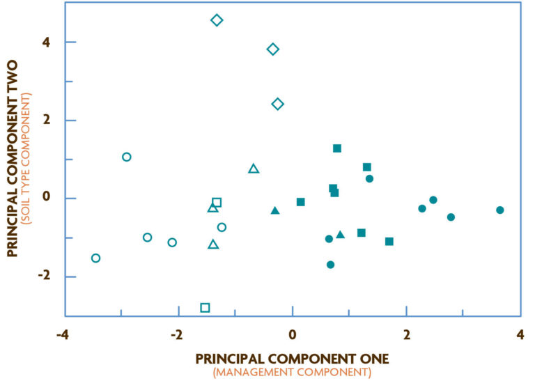
The first two PCs (PC1 and PC2, shown in Figure 4.1) accounted for 31 and 24 percent of the total variance, respectively, based on the loading, which is a calculated coefficient by which each original variable is multiplied to identify an overall component score for each observation. For example, PC1 showed a clear separation of organic and conventional fields and was composed of soil properties likely to be strongly affected by management practices (inorganic nitrogen pools, nitrogen-mineralization potential and electrical conductivity, Table 4.2). Total Kjeldahl nitrogen, exchangeable potassium and pH also contributed significantly to separation along this axis, as indicated by the loadings, which suggested a strong effect of management on these properties (Table 4.2). In contrast, separation of three Vertisols under conventional management occurred along PC2, primarily due to greater clay content with high cation exchange capacity and wet aggregate stability. Organic and conventional fields did not segregate along this axis. Thus, PC2 reflected variation that was mostly associated with differences in soil type among sites.
Based on PCA of the 10 soil variables, the authors identified four distinguishable management categories: fields in organic management for more than three years, fields in organic management for less than three years, conventional fields not on Vertisols, and conventional fields on Vertisols. They then used these categories in a CDA to test the hypothesis that management effects would be more pronounced under long-term (i.e., more than three years) management and to identify which soil variables were most closely associated with these management categories.
CDA is used to test and describe relationships among two or more group categories based on a set of variables (in this case, the 10 soil response variables). With CDA, variation among management categories is maximized while variation within categories is minimized, and the dimensionality of the data set is once again reduced into a smaller set of new variables, now called canonical functions. These newly derived canonical functions describe between-category variation; loadings within canonical functions describe the magnitude and direction of association of an original variable within a described category. Each canonical function (CAN) is a linear combination of independently measured variables and is independent of other canonical functions (Vaylay and van Santen, 2002). In the Drinkwater study, a significant Wilks’ lambda value of 0.37 and a canonical correlation of P = .0001 between the four management categories and the first canonical function (CAN1) indicated that CAN1 explained the differentiation of the management groups (Figure 4.2). The analysis also showed that CAN1 was dominated by large loadings from pH, nitrogen- mineralization potential and Kjeldahl nitrogen and had a negative inorganic nitrogen loading (see Drinkwater et al., 1995 for detailed results of the CDA).
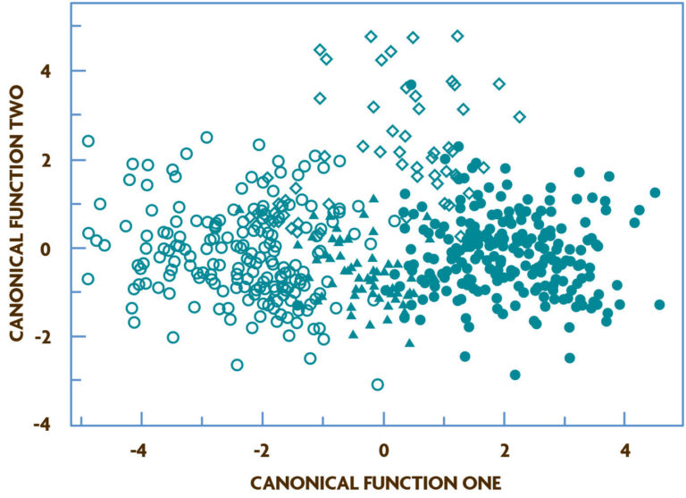
In other words, differences in management-influenced soil properties were greatest between fields that had been managed organically for more than three years and conventional sites not on Vertisols. Fields that were under organic management for three years or less were intermediate. As with PCA, CDA helped reveal which variables were most important for classification into different groups. In this case, total Kjeldahl nitrogen, organic carbon, inorganic nitrogen pools, pH, and electrical conductivity were significant factors in distinguishing between the three groups that remained after fields with confounding soil-type variation were removed. Using multivariate analyses, this study iden-tified key differences in soil properties resulting from these distinct management regimes.
Hierarchical clustering analysis (HCA) is a classification method that produces a set of nested clusters organized as a hierarchical tree, or dendrogram (Figure 4.3). The dendrogram can be viewed on the observational level or as response measures, depending on the research scope (i.e., detailed or general). This flexibility is extremely helpful when examining relationships among entities or subgroups. HCA can reveal patterns that can lead to further hypothesis generation and testing, and it can assist in summarizing data as a precursor to regression, PCA or other classification methods.